¶ Week 5 Lab · Two-sided samples and signed node currents
فارسی · Curriculum · Week 5 guide
Allow about 100 minutes across Thursday and Friday in place of repeated exercises. You need the two Week 5 lessons and Python 3. Use LTspice on your own computer for the simulator comparison if available.
¶ 1 · Predict by hand · 25 minutes
- For f(x) = (x² − 9)/(x − 3), calculate the outputs at 2.99 and 3.01. Record the left-hand and right-hand trends, and the reason there is no sample at 3.
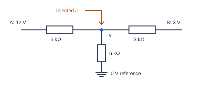
- For the three branches shown below, predict v and the three currents leaving v for J = −4, 0 and 1 mA. Before calculating, predict which case can put the node below ground.
¶ 2 · Generate and compare · 30 minutes
Extract the ZIP. Open lab.py in a Python editor and run it, or run python3 lab.py inside the extracted directory. The script uses the standard library and writes its CSV tables and SVG plots beside itself. Open the SVG files in a browser. The archive includes reference results for comparison.
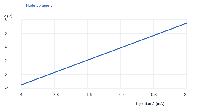
In limit-samples.csv, compare the two rows at distance 0.01 with your predictions. Explain why the agreement supports the trend, and then use the factorization to justify it for every nearby domain point. In node-sweep.csv, find your three J values and check that the current sum equals J. The slope of the v-versus-J graph is 1.5 V/mA.
| J (mA) | v (V) | To A (mA) | To B (mA) | To ground (mA) |
|---|---|---|---|---|
| −4 | −1.5 | −2.25 | −1.5 | −0.25 |
| 0 | 4.5 | −1.25 | 0.5 | 0.75 |
| 1 | 6 | −1 | 1 | 1 |
¶ 3 · Simulator comparison · 25 minutes
Open node-sweep.cir in LTspice and run the DC sweep. Plot V(v) and inspect the three source settings in the table. The current source is declared from 0 to v, so positive J injects into v. The resistors are declared from v to their far terminals, matching the hand current references. Convert A to mA before comparing. If you do not have a working simulator, mark that column pending and finish the Python comparison.
¶ 4 · Readiness checkpoint · 20 minutes
Save your hand predictions, a plot, the three comparison rows and a short correction note. Check four things independently, one point each.
- You can explain why x = 3 is missing even though both branches tend to 6.
- Your signed currents sum to J in all three rows.
- You can explain why the ground branch reverses when v is negative.
- You can reproduce one row without the files, with correct units and arrows.
Revisit any missed item before the Saturday exam.