¶ 2.1 · Limits from graphs and tables
فارسی · Curriculum · Week 5 guide · Course index
¶ Learning goals
Estimate a finite limit from either side of a point, distinguish a limit from a function value, and justify when a two-sided limit does not exist. Use a table to investigate a conjecture, then use the rule or the graph to defend your conclusion. You’ll use these skills next when you learn how limit laws combine simpler limits.
¶ What a limit tells you
Suppose a calibration model gives an output for every input near 3 except exactly 3. We can still ask what outputs the model predicts as the input moves closer to 3. The limit describes that nearby behavior. The value at 3, if the model has one, answers a separate question about a single input.
Write limₓ→ₐ f(x) = L when the outputs approach the same finite number L as x approaches a from either side, with x ≠ a. For the left-hand limit, use inputs x < a. For the right-hand limit, use inputs x > a. The two-sided limit equals L when both one-sided limits exist and equal L. The superscripts in x → a⁻ and x → a⁺ name the approach direction. They do not tell you whether the outputs are positive or negative.
In a table, track the distance |x − a| as well as the output. A useful first pass is to sample at a ± 0.1, a ± 0.01 and a ± 0.001, where the function is defined. Organize the samples by side and keep more digits than the expected difference. A rounded table can hide a small jump. A finite table also cannot rule out behavior between the sample points, so use it to form a hypothesis and turn to the formula to test it.
¶ Example 1 · A missing calibration sample
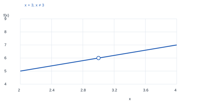
For x ≠ 3, let f(x) = (x² − 9)/(x − 3). Before substituting, factor the numerator as (x − 3)(x + 3). On every input in the original domain, f(x) = x + 3. The simplified rule still represents the original function only where x ≠ 3.
| Side | x | f(x) |
|---|---|---|
| Left | 2.9 | 5.9 |
| Left | 2.99 | 5.99 |
| Right | 3.01 | 6.01 |
| Right | 3.1 | 6.1 |
Both sides approach 6. The factorization explains the pattern for every nearby input: the output error f(x) − 6 is exactly x − 3, so reducing the input error by a factor of ten reduces the output error by the same factor. The limit exists even though the original quotient has no value at 3. Dividing 0 by 0 would not establish any of these facts.
¶ Example 2 · A filled point off the curve
Let g(x) = x + 3 for x ≠ 3 and set g(3) = 8. Draw the same open point at (3, 6), then mark a filled point at (3, 8). The nearby inputs used in Example 1 give exactly the same outputs, so the two-sided limit is still 6. The function value is now 8. If a display reports 8 exactly at input 3, that reading does not change the trend of the nearby calibration data.
¶ Example 3 · A threshold with two different outputs
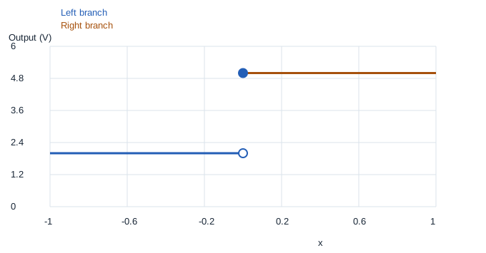
A simplified controller outputs 2 V for x < 0 and 5 V for x ≥ 0. At the threshold, the left-hand limit is 2 V and the right-hand limit is 5 V. The two-sided limit does not exist because the sides disagree. The value at 0 is 5 V, which settles the controller output exactly at the threshold. Changing this single value to 2 V or 3.5 V would leave the two side limits unchanged. In particular, averaging the side limits gives no useful prediction of nearby outputs.
¶ Example 4 · A domain endpoint
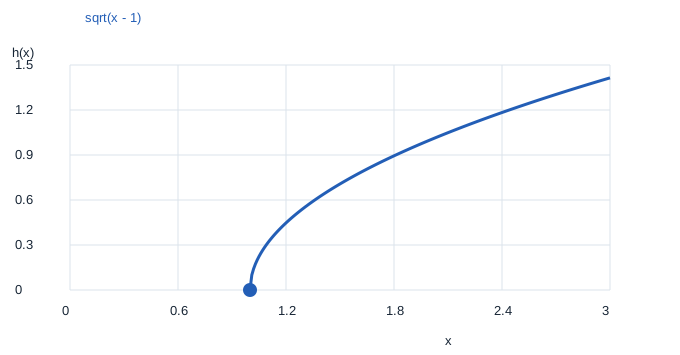
Take h(x) = √(x − 1) over the reals. At x = 1, sample 1.01 and 1.0001. The outputs are 0.1 and 0.01. The right-hand limit is 0 because √(x − 1) becomes arbitrarily small as the positive gap x − 1 shrinks. There are no real domain points to the left of 1, so there is no left-hand approach. Report the right-hand limit explicitly. This lesson uses the two-sided convention for an unqualified limit, so a right-hand approach alone does not establish a two-sided limit at an endpoint.
¶ Troubleshooting your reasoning
- The formula gives 0/0. Check where the original rule is defined. Try factoring, then examine the resulting rule on nearby domain points.
- The graph shows a filled dot. Write the point value on one line and the two side limits on another. Read the trend of each branch.
- The table seems stable. Try points on the other side and examine the domain. Use algebra or an exact branch rule to justify your answer when available.
- The sides disagree. State each side’s result and the reason the two-sided limit fails.
¶ Practice
Do 1–6 without the worked answers. Problems 7–8 are optional extensions.
- Estimate the limit of 2x − 1 at x = 4. Give two samples from each side and justify the result using the output error.
- Find the limit of (x² − 16)/(x − 4) at 4 and state its value at 4 if defined.
- Define the quotient in Problem 2 to equal −1 at 4. What changes?
- For f(x) = 1 when x < 2 and f(x) = 4 otherwise, give both side limits and f(2). Is there a two-sided limit?
- Give the real domain and right-hand limit at 2 for √(x − 2). Explain why a left-hand table is unavailable.
- A sensor rule is x + 1 for x < 0 and 1 − x for x > 0. It has no value at 0. Find both side limits and explain what value would match them.
- Find the side limits of |x − 1|/(x − 1) at 1. Explain the sign on each side.
- The samples at x = −0.1 and 0.1 both equal 2. Compare the possible limits at 0 for f(x) = 2 and g(x) = 1 + 100x². What can the samples establish?
¶ Worked answers
- At 3.9 and 3.99 the outputs are 6.8 and 6.98. At 4.01 and 4.1 they are 7.02 and 7.2. The error is 2(x − 4), which tends to zero from both sides. The limit is 7.
- The quotient equals x + 4 for x ≠ 4, so the limit is 8. The original quotient is undefined at 4.
- Only the point value changes. It becomes −1 and the limit remains 8.
- The left-hand limit is 1, the right-hand limit is 4 and f(2) = 4. The limits disagree, so no two-sided limit exists.
- The real domain is [2, ∞). The square root tends to 0 from the right. The real domain excludes x < 2.
- Each branch tends to 1 as x tends to 0. The limit is 1 and setting f(0) = 1 matches it.
- On the left, |x − 1| = −(x − 1) so the quotient is −1. On the right the quotient is 1. There is no two-sided limit.
- The limits are 2 and 1 respectively. Those two samples agree, but they cannot determine the limit.