¶ Week 6 Lab · Limit samples and source contributions
فارسی · Curriculum · Week 6 guide
Compare a hand prediction, a numerical table, and a circuit simulation. You need the two Week 6 lessons, signed KCL, Python 3, and LTspice for the simulator comparison. The lab takes about 100 minutes and replaces part of Friday's practice.
Download the Python script, LTspice netlist, and reference results
¶ 1 · Predict by hand · 20 minutes
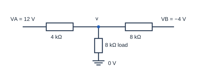
Factor the numerator of q(x) = (x² − 16)/(x − 4). Predict the limit, the domain restriction, and the sample error at x = 3.99 and x = 4.01. For the circuit, draw the two source cases. VA connects to v through 4 kΩ, VB = −4 V through 8 kΩ, and the load is 8 kΩ to ground. Find v at VA = 0, 2, and 12 V. Predict where the load current changes sign.
¶ 2 · Generate and compare · 30 minutes
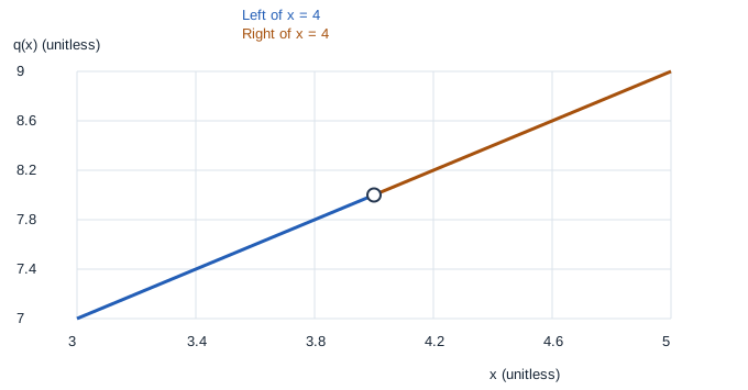
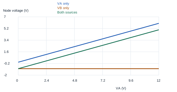
Unzip the files into a writable folder. In a terminal in that folder run python3 lab.py (or py lab.py on Windows). Open quotient.csv and quotient.svg. Both sides should approach 8 and the original formula should have a hole at x = 4. The two samples at distance 0.01 should both have absolute error 0.01. If they differ in the last digits, compare with a tolerance such as 10⁻⁹. Then open source-sweep.csv and source-sweep.svg. Find the A-only slope, the B-only offset, and the zero crossing. Record the three predicted and generated values side by side.
¶ 3 · Compare with LTspice · 30 minutes
Open source-sweep.cir, run it, and plot V(v) and I(RL). The supplied netlist sweeps VA from 0 to 12 V with VB fixed at −4 V. In a copy set VB to 0 and rerun the sweep. For a B-only check set VA to 0, keep VB at −4 V, and replace the sweep with .op. Keep all three resistors in both copies. At each checked input, the both-source voltage should equal the signed sum of the two contributions. If results disagree, check ground, source polarity, and the 4k/8k values. If your installed version cannot run the netlist, recreate it from the diagram or clearly label your comparison as Python-only.
¶ 4 · Readiness and saved work · 20 minutes
- Explain why q(4) is undefined while the limit is 8. The cancellation is valid only off x = 4.
- Explain the zero crossing at VA = 2 V. VA contributes +1 V and VB contributes −1 V. The load current is zero, but the source branches still carry current.
- At VA = 12 V check that v = 5 V and I(RL) = 0.625 mA. The load power is 3.125 mW. The sum of powers from separate runs is 4.625 mW because squaring separately omits the cross term.
Save both CSVs, a graph with units, your hand table, and a short note on any discrepancy. Identify the plots you generated and any reference plots you used.