¶ Week 4 lab · Loaded Divider and Practical Checkpoint
Study guide · Curriculum · فارسی
¶ Purpose and time budget
Complete a first practical checkpoint: predict, simulate and explain a loaded divider using KCL, KVL and power balance. This closes the first month’s lab sequence. It is not the cumulative Month 3 assessment, which must also cover later limits, derivatives and the DC objectives taught by then. Allow 110–150 minutes during Thursday/Friday, replacing routine repeated exercises.
¶ Predict the unloaded and loaded circuit · 25 minutes
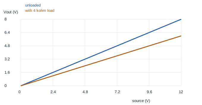
An ideal source drives R1=2 kΩ above R2=4 kΩ. With no load, Vout=Vs × 4/(2+4). Add a 4 kΩ load in parallel with R2. The lower equivalent becomes 2 kΩ, making Vout=Vs/2. Predict both outputs for source values 3, 6 and 12 V. At 12 V also predict all three resistor currents, their powers and the source power.
¶ Python calculation and graph · 20 minutes
- Download the Week 4 lab package and extract the ZIP archive.
- Open
lab.pyin your Python editor and run it, or runpython3 lab.pyfrom that extracted folder. Python 3 is required; no extra packages are needed. - Read the printed checks. Open the generated SVG graphs in your browser and CSV tables in your preferred spreadsheet.
The package includes reference plots for comparison. Running lab.py regenerates them; opening a reference plot alone does not mean you have run the experiment.
Open divider.svg and checkpoint.csv. The script checks current and power balance at every source setting, not just the final point. Its KCL_error_A and power_error_W columns should be zero or tiny numerical roundoff values. A successful assertion checks the stated ideal model; it does not prove that every real divider has these exact component values.

¶ LTspice loaded and unloaded comparison · 30 minutes
Install or open LTspice from Analog Devices. In LTspice, use File → Open to open circuit.cir from the extracted package. The file is a text netlist, so you do not need to draw a schematic first. Run it, then use Add Trace in the waveform window to select the named traces below. If your file picker filters extensions, choose all files. The circuit diagram below explains the same node connections as the file. Only software simulations are assigned.
Mogissi Academy Week 4 - loaded divider checkpoint
V1 vin 0 0
R1 vin out 2k
R2 out 0 4k
RLOAD out 0 4k
.dc V1 0 12 0.5
.save V(vin) V(out) I(R1) I(R2) I(RLOAD)
.end
Run and plot V(out), I(R1), I(R2) and I(RLOAD). Then save a second copy as unloaded.cir, delete only the RLOAD line, remove I(RLOAD) from the .save line, and run again. Retain the first loaded file so you can compare both results. Read each output at the same source settings. A DC sweep is a sequence of steady operating points, not a time-domain charging experiment.
¶ Expected checks
| Source | Unloaded output | Loaded output |
|---|---|---|
| 3 V | 2 V | 1.5 V |
| 6 V | 4 V | 3 V |
| 12 V | 8 V | 6 V |
At 12 V in the loaded circuit, I(R1)=3 mA, I(R2)=1.5 mA and I(RLOAD)=1.5 mA. KCL gives 3−1.5−1.5=0 mA. KVL gives 12−6−6=0 V. The upper resistor absorbs 18 mW and the two lower branches 9 mW each, matching 36 mW supplied by the source. Loading reduces the output from 8 V to 6 V, a 25% decrease relative to the unloaded value.
¶ Week 4 practical checkpoint · 20 points
Complete this explanation without reading the answer table first. Award 5 points for each item, then correct every missed part.
- Draw the actual nodes and show why R2 and RLOAD are parallel.
- Derive the two voltage ratios rather than quoting a memorised divider formula.
- Verify KCL, KVL and power balance at 12 V with units.
- Explain why the output changes when the load changes, and why this circuit is not a regulated supply.
Save one page containing the diagram, three-row hand/Python/LTspice comparison, plots and your explanation. A score of 16/20 is a suggested review target, not a course credit. Any incorrect node connection, unit conversion or conservation check needs correction even if your total score is high. Keep this report for the Month 3 cumulative checkpoint. The Saturday written exam is separate.