¶ Week 3 lab · Decay Graphs and Meter Loading
Study guide · Curriculum · فارسی
¶ Purpose and time budget
Investigate a meter that changes the circuit it measures, and generate an exponential-decay graph. Use 100–140 minutes across Thursday and Friday. Reuse Week 2’s LTspice setup. This lab is based on series/parallel calculations already taught; the full divider derivation follows in Week 4.
¶ Predict three cases · 25 minutes
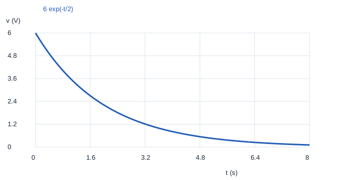
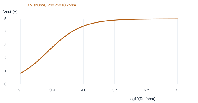
An ideal 10 V source feeds two series 10 kΩ resistors. The unloaded midpoint is 5 V. Put a hypothetical meter resistance Rm in parallel with the lower resistor. For Rm equal to 10 kΩ, 100 kΩ and 10 MΩ, first find Rp=R2 Rm/(R2+Rm), then total current and the voltage across Rp. Compute signed error as (reading−5)/5 × 100%. Separately, predict the half-value time and the value at 2 s for v(t)=6 exp(−t/2) V.
¶ Generate and read the graphs · 20 minutes
- Download the Week 3 lab package and extract the ZIP archive.
- Open
lab.pyin your Python editor and run it, or runpython3 lab.pyfrom that extracted folder. Python 3 is required; no extra packages are needed. - Read the printed checks. Open the generated SVG graphs in your browser and CSV tables in your preferred spreadsheet.
The package includes reference plots for comparison. Running lab.py regenerates them; opening a reference plot alone does not mean you have run the experiment.
Open decay.svg, loading.svg and the CSV tables. The loading graph uses x=log10(Rm/Ω), so x=3, 4, 5, 6 and 7 represent 1 kΩ, 10 kΩ, 100 kΩ, 1 MΩ and 10 MΩ. Equal horizontal steps multiply resistance by ten. The curve’s vertical coordinate remains an ordinary voltage; it is not a logarithm of voltage.

¶ Repeat the measurement in LTspice · 30 minutes
Install or open LTspice from Analog Devices. In LTspice, use File → Open to open circuit.cir from the extracted package. The file is a text netlist, so you do not need to draw a schematic first. Run it, then use Add Trace in the waveform window to select the named traces below. If your file picker filters extensions, choose all files. The circuit diagram below explains the same node connections as the file. Only software simulations are assigned.
Mogissi Academy Week 3 - voltmeter loading
V1 vin 0 0
R1 vin out 10k
R2 out 0 10k
RMETER out 0 {RM}
.step param RM list 10k 100k 10Meg
.dc V1 0 10 0.5
.save V(vin) V(out) I(R1) I(R2) I(RMETER)
.end
Plot V(out). The .step instruction repeats the DC sweep for three constant meter resistances. Use the step legend or select one run at a time to identify which resistance produced each line. Read all three outputs at the same 10 V source setting. Node 0 is the common reference. The RMETER branch is a simplified voltmeter input model; it is not a second independent source. In SPICE, write 10Meg for ten megaohms: M is interpreted as milli, not mega.
¶ Expected checks
| Meter input | Reading at 10 V source | Signed loading error |
|---|---|---|
| 10 kΩ | 3.33333 V | −33.3333% |
| 100 kΩ | 4.76190 V | −4.7619% |
| 10 MΩ | 4.99750 V | about −0.0500% |
The decay half-value time is 2 ln 2 ≈ 1.3863 s, and v(2)=6/e ≈ 2.2073 V. A meter can be accurately calibrated yet still lower the circuit voltage through loading. Instrument accuracy and loading error are different effects.
¶ Deliverables and checkpoint · 25 minutes
Keep both Python graphs, a sweep showing the three meter cases, and a table comparing hand, Python and LTspice readings. Explain the log axis and the SPICE Meg suffix. State which meter gives the smallest loading error and why. Recalculate one case from the parallel equivalent without looking at the solution. Do not claim simulation agreement for a run you have not performed.