¶ Week 2 lab · Waveforms and Resistor DC Sweeps
Study guide · Curriculum · فارسی
¶ Purpose and time budget
Compare hand predictions, Python graphs and an LTspice DC sweep. Revisit frequency and phase using a time graph, then investigate two ohmic resistors across the same source. Allow 100–140 minutes across Thursday and Friday within your normal study budget. Installing software for the first time can take extra setup time; use the supplied graphs to complete the reasoning if needed and record the simulation as pending.
¶ Predict first · 20 minutes
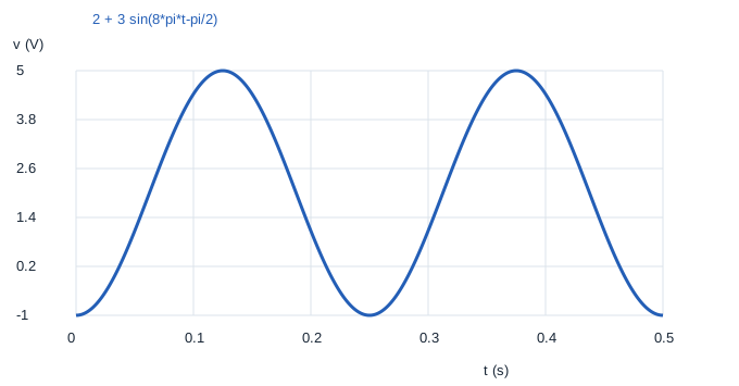
For v(t)=2+3 sin(8πt−π/2) V, predict amplitude, frequency, period, range and v(0). Separately, place 2 kΩ and 4 kΩ in parallel across an ideal variable DC source. Calculate both branch currents and powers at source values 2, 6 and 12 V. These are two different experiments: the sinusoid is a mathematical time signal, while the DC sweep changes a steady source setting.
¶ Python graphs · 20 minutes
- Download the Week 2 lab package and extract the ZIP archive.
- Open
lab.pyin your Python editor and run it, or runpython3 lab.pyfrom that extracted folder. Python 3 is required; no extra packages are needed. - Read the printed checks. Open the generated SVG graphs in your browser and CSV tables in your preferred spreadsheet.
The package includes reference plots for comparison. Running lab.py regenerates them; opening a reference plot alone does not mean you have run the experiment.
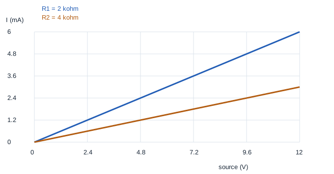
Open wave.svg, sweep.svg and their CSV tables. The waveform should complete two cycles in 0.5 s. The DC current curves should be straight lines through the origin, with the 2 kΩ branch carrying twice the 4 kΩ branch current at the same voltage.

¶ LTspice DC sweep · 30 minutes
Install or open LTspice from Analog Devices. In LTspice, use File → Open to open circuit.cir from the extracted package. The file is a text netlist, so you do not need to draw a schematic first. Run it, then use Add Trace in the waveform window to select the named traces below. If your file picker filters extensions, choose all files. The circuit diagram below explains the same node connections as the file. Only software simulations are assigned.
Mogissi Academy Week 2 - resistor DC sweep
V1 vin 0 0
R1 vin 0 2k
R2 vin 0 4k
.dc V1 0 12 0.5
.save V(vin) I(R1) I(R2)
.end
Run the analysis and add traces I(R1) and I(R2). The horizontal axis is the swept source voltage in volts, not time. Both resistors connect between vin and node 0, so both receive the full source voltage. The resistor current reference follows the listed node order from vin to 0. If you inspect I(V1), its sign is negative while the source supplies power because SPICE defines source current entering its positive terminal.
¶ Expected checks
| Source | I(R1), 2 kΩ | I(R2), 4 kΩ | Total resistor power |
|---|---|---|---|
| 2 V | 1 mA | 0.5 mA | 3 mW |
| 6 V | 3 mA | 1.5 mA | 27 mW |
| 12 V | 6 mA | 3 mA | 108 mW |
For the time signal, amplitude is 3 V, frequency 4 Hz, period 0.25 s, range [−1,5] V and v(0)=−1 V. A different simulator step size changes the density of plotted points, not the ideal resistor law.
¶ Deliverables and checkpoint · 30 minutes
Save a labeled waveform graph, a resistor sweep screenshot or exported plot, and a three-row table comparing hand, Python and LTspice results. If LTspice has not run, mark that column pending rather than claiming agreement. Explain the difference between the two horizontal axes, why doubling resistance halves current at fixed voltage, and why power grows quadratically with source voltage. Use P=V²/R to verify one row. Correct any mA-to-A mistake before the Saturday exam.